Search Space Representation

This module provides common building blocks to define a search space.

Search spaces are defined using dictionaries, where the keys are the parameter names and the values their distribution. For example, defining a two parameter search space is done as follow

space = {"x": uniform(-5, 5),
         "y": quantized_uniform(-2, 3, 0.5)}

A conditional search space can be seen as a tree, where each condition defines a subtree. For example, in the next figure, three search spaces are presented.

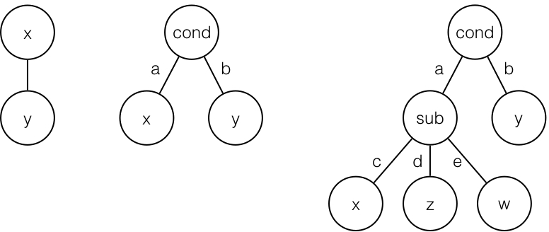
The left tree is the simple two parameter search space defined earlier. The middle tree defines a conditional search space with a single root condition. Two subspaces exist in this search space, one when the condition is a the other when the condition is b. Defining such a search space is done using a list of dictionaries as follow

space = [{"cond": "a", "x": uniform(-5, 5)},
         {"cond": "b", "y": quantized_uniform(-2, 3, 0.5)}]

The right most tree has two conditions one at its root and another one when the root condition is a. It has a total of four subspaces. Defining such a search space is done using a hierarchy of dictionaries as follow

space = [{"cond": "a", "sub": {"c": {"x": uniform(-5, 5)},
                               "d": {"z": log(-5, 5, 10)},
                               "e": {"w": quantized_log(-2, 7, 1, 10)}}},
         {"cond": "b", "y": quantized_uniform(-2, 3, 0.5)}

Note that lists can only be used at the root of conditional search spaces, sub-conditions must use the dictionary form. Moreover, it is not necessary to use the same parameter name for root conditions. For example, the following is a valid search space

space = [{"cond": "a", "x": uniform(-5, 5)},
         {"spam": "b", "y": quantized_uniform(-2, 3, 0.5)}]

The only restriction is that each search space must have a unique combination of conditional parameters and values, where conditional parameters have non-distribution values. Finally, one and only one subspace can be defined without condition as follow

space = [{"x": uniform(-5, 5)},
         {"cond": "b", "y": quantized_uniform(-2, 3, 0.5)}]

If two or more subspaces share the same conditional key (set of parameters and values) an AssertionError will be raised uppon building the search space specifying the erroneous key.

class chocolate.Space(spaces)

Representation of the search space.

Encapsulate a multidimentional search space defined on various distributions. Remind that order in standard python dictionary is undefined, thus the keys of the input dictionaries are sorted() and put in OrderedDict s for reproductibility.

Parameters:spaces – A dictionary or list of dictionaries of parameter names to their distribution. When a list of multiple dictionaries is provided, the structuring elements of these items must define a set of unique choices. Structuring elements are defined using non-distribution values. See examples below. Raises:AssertionError – When two keys at the same level are equal.

An instance of a space is a callable object wich will return a valid parameter set provided a vector of numbers in the half-open uniform distribution \([0, 1)\).

The number of distinc dimensions can be queried with the len() function. When a list of dictionaries is provided, this choice constitute the first dimension and each subsequent conditional choice is also a dimension.

Examples

Here is how a simple search space can be defined and the parameters can be retrieved

In [2]: s = Space({"learning_rate": uniform(0.0005, 0.1),
                   "n_estimators" : quantized_uniform(1, 11, 1)})

In [3]: s([0.1, 0.7])
Out[3]: {'learning_rate': 0.01045, 'n_estimators': 8}

A one level conditional multidimentional search space is defined using a list of dictionaries. Here the choices are a SMV with linear kernel and a K-nearest neighbor as defined by the string values. Note the use of class names in the space definition.

In [2]: from sklearn.svm import SVC

In [3]: from sklearn.neighbors import KNeighborsClassifier

In [4]: s = Space([{"algo": SVC, "kernel": "linear",
                        "C": log(low=-3, high=5, base=10)},
                   {"algo": KNeighborsClassifier,
                        "n_neighbors": quantized_uniform(low=1, high=20, step=1)}])

The number of dimensions of such search space can be retrieved with the len() function.

In [5]: len(s)
Out[5]: 3

As in the simple search space a valid parameter set can be retrieved by querying the space object with a vector of length equal to the full search space.

In [6]: s([0.1, 0.2, 0.3])
Out[6]:
{'C': 0.039810717055349734,
 'algo': sklearn.svm.classes.SVC,
 'kernel': 'linear'}

In [7]: s([0.6, 0.2, 0.3])
Out[7]:
{'algo': sklearn.neighbors.classification.KNeighborsClassifier,
 'n_neighbors': 6}

Internal conditions can be modeled using nested dictionaries. For example, the SVM from last example can have different kernels. The next search space will share the C parameter amongst all SVMs, but will branch on the kernel type with their individual parameters.

In [2]: s = Space([{"algo": "svm",
                    "C": log(low=-3, high=5, base=10),
                    "kernel": {"linear": None,
                                "rbf": {"gamma": log(low=-2, high=3, base=10)}}},
                   {"algo": "knn",
                        "n_neighbors": quantized_uniform(low=1, high=20, step=1)}])

In [3]: len(s)
Out[3]: 5

In [4]: x = [0.1, 0.2, 0.7, 0.4, 0.5]

In [5]: s(x)
Out[5]: {'C': 0.039810717055349734, 'algo': 'svm', 'gamma': 1.0, 'kernel': 'rbf'}

names(unique=True)

Returns unique sequential names meant to be used as database column names.

Parameters:unique – Whether or not to return unique mangled names. Subspaces will still be mangled.

Examples

If the length of the space is 2 as follow

In [2]: s = Space({"learning_rate": uniform(0.0005, 0.1),
                   "n_estimators" : quantized_uniform(1, 11, 1)})

In [3]: s.names()
Out[3]: ['learning_rate', 'n_estimators']

While in conditional spaces, if the length of the space is 5 (one for the choice od subspace and four independent parameters)

In [4]: s = Space([{"algo": "svm", "kernel": "linear",
                        "C": log(low=-3, high=5, base=10)},
                   {"algo": "svm", "kernel": "rbf",
                        "C": log(low=-3, high=5, base=10),
                        "gamma": log(low=-2, high=3, base=10)},
                   {"algo": "knn",
                        "n_neighbors": quantized_uniform(low=1, high=20, step=1)}])

In [5]: s.names()
Out[5]:
['_subspace',
 'algo_svm_kernel_linear_C',
 'algo_svm_kernel_rbf_C',
 'algo_svm_kernel_rbf_gamma',
 'algo_knn_n_neighbors']

When using methods or classes as parameter values for conditional choices the output might be a little bit more verbose, however the names are still there.

In [6]: s = Space([{"algo": SVC,
                    "C": log(low=-3, high=5, base=10),
                    "kernel": {"linear": None,
                                "rbf": {"gamma": log(low=-2, high=3, base=10)}}},

                   {"algo": KNeighborsClassifier,
                        "n_neighbors": quantized_uniform(low=1, high=20, step=1)}])

In [7]: s.names()
Out[7]:
['_subspace',
 'algo_<class sklearn_svm_classes_SVC>_C',
 'algo_<class sklearn_svm_classes_SVC>_kernel__subspace',
 'algo_<class sklearn_svm_classes_SVC>_kernel_kernel_rbf_gamma',
 'algo_<class sklearn_neighbors_classification_KNeighborsClassifier>_n_neighbors']

isactive(x)

Checks within conditional subspaces if, with the given vector, a parameter is active or not.

Parameters:x – A vector of numbers in the half-open uniform distribution \([0, 1)\). Returns:A list of booleans telling is the parameter is active or not.

Example

When using conditional spaces it is often necessary to assess quickly what dimensions are active according to a given vector. For example, with the following conditional space

In [2]: s = Space([{"algo": "svm",
                    "C": log(low=-3, high=5, base=10),
                    "kernel": {"linear": None,
                                "rbf": {"gamma": log(low=-2, high=3, base=10)}}},
                   {"algo": "knn",
                        "n_neighbors": quantized_uniform(low=1, high=20, step=1)}])
In [3]: s.names()
Out[3]:
['_subspace',
 'algo_svm_C',
 'algo_svm_kernel__subspace',
 'algo_svm_kernel_kernel_rbf_gamma',
 'algo_knn_n_neighbors']

In [4]: x = [0.1, 0.2, 0.7, 0.4, 0.5]

In [5]: s(x)
Out[5]: {'C': 0.039810717055349734, 'algo': 'svm', 'gamma': 1.0, 'kernel': 'rbf'}

In [6]: s.isactive(x)
Out[6]: [True, True, True, True, False]

In [6]: x = [0.6, 0.2, 0.7, 0.4, 0.5]

In [8]: s(x)
Out[8]: {'algo': 'knn', 'n_neighbors': 10}

In [9]: s.isactive(x)
Out[9]: [True, False, False, False, True]

steps()

Returns the steps size between each element of the space dimensions. If a variable is continuous the returned stepsize is None.

isdiscrete()

Returns whether or not this search space has only discrete dimensions.

subspaces()

Returns every valid combinaition of conditions of the tree- structured search space. Each combinaition is a list of length equal to the total dimensionality of this search space. Active dimensions are either a fixed value for conditions or a Distribution for optimizable parameters. Inactive dimensions are None.

Example

The following search space has 3 possible subspaces

In [2]: s = Space([{"algo": "svm",
                    "C": log(low=-3, high=5, base=10),
                    "kernel": {"linear": None,
                                "rbf": {"gamma": log(low=-2, high=3, base=10)}}},
                   {"algo": "knn",
                        "n_neighbors": quantized_uniform(low=1, high=20, step=1)}])

In [3]: s.names()
Out[3]:
['_subspace',
 'algo_svm_C',
 'algo_svm_kernel__subspace',
 'algo_svm_kernel_kernel_rbf_gamma',
 'algo_knn_n_neighbors']

In [4]: s.subspaces()
Out[4]:
[[0.0, log(low=-3, high=5, base=10), 0.0, None, None],
 [0.0, log(low=-3, high=5, base=10), 0.5, log(low=-2, high=3, base=10), None],
 [0.5, None, None, None, quantized_uniform(low=1, high=20, step=1)]]

class chocolate.Distribution

Base class for every Chocolate distributions.

class chocolate.ContinuousDistribution

Base class for every Chocolate continuous distributions.

class chocolate.QuantizedDistribution

Base class for every Chocolate quantized distributions.

class chocolate.uniform(low, high)

Uniform continuous distribution.

Representation of the uniform continuous distribution in the half-open interval \([\text{low}, \text{high})\).

Parameters:

• low – Lower bound of the distribution. All values will be greater or equal than low.
• high – Upper bound of the distribution. All values will be lower than high.

__call__(x)

Transforms x a uniform number taken from the half-open continuous interval \([0, 1)\) to the represented distribution.

Returns:The corresponding number in the half-open interval \([\text{low}, \text{high})\).

class chocolate.quantized_uniform(low, high, step)

Uniform discrete distribution.

Representation of the uniform continuous distribution in the half-open interval \([\text{low}, \text{high})\) with regular spacing between samples. If \(\left\lceil \frac{\text{high} - \text{low}}{step} \right\rceil \neq \frac{\text{high} - \text{low}}{step}\), the last interval will have a different probability than the others. It is preferable to use \(\text{high} = N \times \text{step} + \text{low}\) where \(N\) is a whole number.

Parameters:

• low – Lower bound of the distribution. All values will be greater or equal than low.
• high – Upper bound of the distribution. All values will be lower than high.
• step – The spacing between each discrete sample.

__call__(x)

Transforms x, a uniform number taken from the half-open continuous interval \([0, 1)\), to the represented distribution.

Returns:The corresponding number in the discrete half-open interval \([\text{low}, \text{high})\) alligned on step size. If the output number is whole, this method returns an int otherwise a float.

__iter__()

Iterate over all possible values of this discrete distribution in the \([0, 1)\) space. This is the same as

numpy.arange(0, 1, step / (high - low))

__getitem__(i)

Retrieve the i th value of this distribution in the \([0, 1)\) space.

__len__()

Get the number of possible values for this distribution.

class chocolate.log(low, high, base)

Logarithmic uniform continuous distribution.

Representation of the logarithmic uniform continuous distribution in the half-open interval \([\text{base}^\text{low}, \text{base}^\text{high})\).

Parameters:

• low – Lower bound of the distribution. All values will be greater or equal than \(\text{base}^\text{low}\).
• high – Upper bound of the distribution. All values will be lower than \(\text{base}^\text{high}\).
• base – Base of the logarithmic function.

__call__(x)

Transforms x, a uniform number taken from the half-open continuous interval \([0, 1)\), to the represented distribution.

Returns:The corresponding number in the discrete half-open interval \([\text{base}^\text{low}, \text{base}^\text{high})\) alligned on step size. If the output number is whole, this method returns an int otherwise a float.

class chocolate.quantized_log(low, high, step, base)

Logarithmic uniform discrete distribution.

Representation of the logarithmic uniform discrete distribution in the half-open interval \([\text{base}^\text{low}, \text{base}^\text{high})\). with regular spacing between sampled exponents.

Parameters:

• low – Lower bound of the distribution. All values will be greater or equal than \(\text{base}^\text{low}\).
• high – Upper bound of the distribution. All values will be lower than \(\text{base}^\text{high}\).
• step – The spacing between each discrete sample exponent.
• base – Base of the logarithmic function.

__call__(x)

Transforms x, a uniform number taken from the half-open continuous interval \([0, 1)\), to the represented distribution.

Returns:The corresponding number in the discrete half-open interval \([\text{base}^\text{low}, \text{base}^\text{high})\) alligned on step size. If the output number is whole, this method returns an int otherwise a float.

__iter__()

Iterate over all possible values of this discrete distribution in the \([0, 1)\) space. This is the same as

numpy.arange(0, 1, step / (high - low))

__getitem__(i)

Retrieve the i th value of this distribution in the \([0, 1)\) space.

__len__()

Get the number of possible values for this distribution.

class chocolate.choice(values)

Uniform choice distribution between non-numeric samples.

Parameters:values – A list of choices to choose uniformly from.

__call__(x)

Transforms x, a uniform number taken from the half-open continuous interval \([0, 1)\), to the represented distribution.

Returns:The corresponding choice from the entered values.

__iter__()

Iterate over all possible values of this discrete distribution in the \([0, 1)\) space. This is the same as

numpy.arange(0, 1, step / (high - low))

__getitem__(i)

Retrieve the i th value of this distribution in the \([0, 1)\) space.

__len__()

Get the number of possible values for this distribution.